


ינהאַלט
We have previously explained to beginners how to use the basic functions of VLOOKUP (English VLOOKUP, the abbreviation stands for “vertical lookup function”). And experienced users were shown several more complicated formulas.
And in this article we will try to give information about another method of working with vertical search.
You may be wondering: “Why is this necessary?”. And this is necessary in order to show all possible search methods. In addition, numerous VLOOKUP restrictions often prevent obtaining the desired result. In this regard, INDEX( ) MATCH( ) is much more functional and diverse, and they also have fewer restrictions.
Basics INDEX MATCH
Since the purpose of this guide is to show how good this feature is, we Let’s look at the basic information regarding the principles of its operation. And we will show examples, and also consider why, it is better than VLOOKUP ().
INDEX Function Syntax and Usage
This function helps in finding the desired value among the specified search areas based on the column or line number. Syntax:
=INDEX(array, row number, column number):
- array – the area in which the search will take place;
- line number – the number of the line to be searched in the specified array. If the row number is unknown, the column number must be specified;
- column number – the number of the column to be found in the specified array. If the value is unknown, a line number is required.
An example of a simple formula:
=INDEX(A1:S10,2,3)
The function will search in the range from A1 to C10. The numbers show which row (2) and column (3) to show the desired value from. The result will be cell C2.
Pretty simple, right? But when you work with real documents, you are unlikely to have information regarding column numbers or cells. That’s what the MATCH() function is for.
MATCH Function Syntax and Usage
The MATCH() function searches for the desired value and shows its approximate number in the specified search area.
The searchpos() syntax looks like this:
=MATCH(value to lookup, array to lookup, match type)
- search value – the number or text to be found;
- searched array – the area where the search will take place;
- match type – specifies whether to look for the exact value or the values closest to it:
- 1 (or no value specified) – returns the largest value that is equal to or less than the value that was specified;
- 0 – shows an exact match with the searched value. In the combination INDEX() MATCH() you will almost always need an exact match, so we write 0;
- -1 – Shows the smallest value that is greater than or equal to the value specified in the formula. Sorting is carried out in descending order.
For example, in the range B1:B3 New York, Paris, London are registered. The formula below will show the number 3 because London is third on the list:
=EXPOSE(London,B1:B3,0)
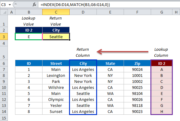
How to work with the INDEX MATCH function
You have probably already begun to understand the principle by which the joint work of these functions is built. In short, then INDEX() searches for the desired value among the specified rows and columns. And MATCH() shows the numbers of these values:
=INDEX(column from which the value is returned, MATCH(value to search, column to search in, 0))
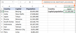
Still having a hard time understanding how it works? Maybe an example will explain better. Suppose you have a list of world capitals and their population:
In order to find out the size of the population of a certain capital, for example, the capital of Japan, we use the following formula:
=INDEX(C2:C10, MATCH(Japan, A2:A10,0))
דערקלערונג:
- The MATCH() function looks for the value – “Japan” in the array A2:A10 and returns the number 3, because Japan is the third value in the list.
- This figure goes toline number” in the INDEX() formula and tells the function to print a value from this row.
So the above formula becomes the standard formula INDEX(C2:C10,3). The formula searches from cells C2 to C10 and returns data from the third cell in this range, that is, C4, because the countdown starts from the second row.
Do not want to prescribe the name of the city in the formula? Then write it in any cell, say F1, and use it as a reference in the MATCH() formula. And you end up with a dynamic search formula:
=ИНДЕКС(С2:С10, ПОИСКПОЗ( )(F1,A2:A10,0))
וויכטיק! Number of lines in מענגע INDEX() must be the same as the number of rows in considered array in MATCH(), otherwise you will get the wrong result.
Wait a minute, why not just use the VLOOKUP() formula?
=VLOOKUP(F1, A2:C10, 3, False)
What’s the point of wasting time trying to figure out all these complexities of INDEX MATCH?
In this case, it doesn’t matter which function to use. This is just an example to understand how the INDEX() and MATCH() functions work together. Other examples will show what these functions are capable of in situations where the VLOOKUP is powerless.
INDEX MATCH or VLOOKUP
When deciding which search formula to use, many agree that INDEX() and MATCH() are vastly superior to VLOOKUP. However, many people still use VLOOKUP(). Firstly, VLOOKUP() is simpler, and secondly, users do not fully understand all the advantages of working with INDEX() and MATCH(). Without this knowledge, no one will agree to spend their time studying a complex system.
Here are the key advantages of INDEX() and MATCH() over VLOOKUP():
- Search from right to left. VLOOKUP() cannot search from right to left, so the values you are looking for must always be in the leftmost columns of the table. But INDEX() and MATCH() can handle this without a problem. This article will tell you what it looks like in practice: how to find the desired value on the left side.
- Safe addition or removal of columns. The VLOOKUP() formula shows incorrect results when removing or adding columns because VLOOKUP() needs the exact column number to be successful. Naturally, when columns are added or removed, their numbers also change.
And in the INDEX() and MATCH() formulas, a range of columns is specified, not individual columns. As a result, you can safely add and remove columns without having to update the formula each time.
- No limits on search volumes. When using VLOOKUP(), the total number of search criteria must not exceed 255 characters or you will get a #VALUE! So if your data contains a large number of characters, INDEX() and MATCH() are the best option.
- High processing speed. If your tables are relatively small, then you are unlikely to notice any difference. But, if the table contains hundreds or thousands of rows, and, accordingly, there are hundreds and thousands of formulas, INDEX () and MATCH () will cope much faster than VLOOKUP (). The fact is that Excel will process only the columns specified in the formula, instead of processing the entire table.
The performance impact of VLOOKUP() will be especially noticeable if your worksheet contains a large number of formulas like VLOOKUP() and SUM(). Separate checks of the VLOOKUP() functions are required to parse each value in an array. So Excel has to process a huge amount of information, and this slows down the work significantly.
Formula Examples
We have already figured out the usefulness of these functions, so we can move on to the most interesting part: the application of knowledge in practice.
Formula to search from right to left
As already mentioned, VLOOKUP cannot perform this form of search. So, if the desired values are not in the leftmost column, VLOOKUP() will not produce a result. The INDEX() and MATCH() functions are more versatile, and the location of the values does not play a big role for them to work.
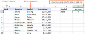
For example, we will add a rank column to the left side of our table and try to figure out what rank in terms of population the capital of Our Country occupies.
In cell G1, we write the value to be found, and then use the following formula to search in the range C1:C10 and return the corresponding value from A2:A10:
=ИНДЕКС(А2:А10, ПОИСКПОЗ(G1,C1:C10,0))
פּינטלעך. If you plan to use this formula for multiple cells, make sure you fix the ranges using absolute addressing (for example, $A$2: $A$10 and $C$2: 4C$10).
INDEX MORE EXPOSED MORE EXPOSED to search in columns and rows
In the above examples, we have used these functions as a replacement for VLOOKUP() to return values from a predefined range of rows. But what if you need to do a matrix or two-sided search?
It sounds complicated, but the formula for such calculations is similar to the standard INDEX() MATCH() formula, with only one difference: the MATCH() formula must be used twice. The first time to get the row number, and the second time to get the column number:
=INDEX(array, MATCH(vertical search value, search column, 0), MATCH(horizontal search value, search row, 0))
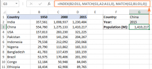
Let’s look at the table below and try to make a formula INDEX() EXPRESS() EXPRESS() in order to display demographics in a specific country for a selected year.
The target country is in cell G1 (vertical lookup) and the target year is in cell G2 (horizontal lookup). The formula will look like this:
=ИНДЕКС(B2:D11, ПОИСКПОЗ(G1,A2:A11,0), ПОИСКПОЗ(G2,B1:D1,0))
ווי דעם פאָרמולע אַרבעט
As with any other complex formulas, they are easier to understand by breaking them down into individual equations. And then you can understand what each individual function does:
- MATCH(G1,A2:A11,0) – looks for a value (G1) in the range A2:A11 and shows the number of this value, in our case it is 2;
- SEARCH(G2,B1:D1,0) – looks for a value (G2) in the range B1:D1. In this case, the result was 3.
The found row and column numbers are sent to the corresponding value in the INDEX() formula:
=INDEX(B2:D11,2,3)
As a result, we have a value that is in a cell at the intersection of 2 rows and 3 columns in the range B2:D11. And the formula shows the desired value, which is in cell D3.
Search by multiple conditions with INDEX and MATCH
If you’ve read our guide to VLOOKUP(), you’ve probably tried multiple search formulas. But this search method has one significant limitation – the need to add an auxiliary column.
But the good news is that With INDEX() and MATCH() you can search for multiple conditions without having to edit or change your worksheet.
Here is the general multi-condition search formula for INDEX() MATCH():
{=ИНДЕКС(диапазон поиска, ПОИСКПОЗ(1,условие1=диапазон1)*(условвие2=диапазон2),0))}
The note: this formula must be used together with the keyboard shortcut CTRL+SHIFT+ENTER.
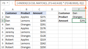
Suppose you need to find the value you are looking for based on 2 conditions: קוינע и פּראָדוקט.
This requires the following formula:
=ИНДЕКС(С2:С10, ПОИСКПОЗ(1,(F1=A2:A10)*(F2=B1:B10),0))
In this formula, C2:C10 is the range in which the search will take place, F1 – this condition, A2:A10 — is the range to compare the condition, F2 – condition 2, וו2:וו10 – range for comparison of condition 2.
Do not forget to press the combination at the end of the work with the formula קטרל + יבעררוק + אַרייַן – Excel will automatically close the formula with curly braces, as shown in the example:
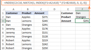
If you do not want to use an array formula for your work, then add another INDEX() to the formula and press ENTER, it will look like in the example:
How these formulas work
This formula works in the same way as the standard INDEX() MATCH() formula. To search for multiple conditions, you simply create multiple False and True conditions that represent the correct and incorrect individual conditions. And then these conditions apply to all corresponding elements of the array. The formula converts the False and True arguments to 0 and 1, respectively, and outputs an array where 1 is the matching values that were found in the string. MATCH() will find the first value that matches 1 and pass it to the INDEX() formula. And it, in turn, will return the already desired value in the specified line from the desired column.
A formula without an array depends on the ability of INDEX() to handle them on its own. The second INDEX() in the formula matches falsy (0), so it passes the entire array with those values to the MATCH() formula.
This is a rather lengthy explanation of the logic behind this formula. For more information read the article “INDEX MATCH with multiple conditions'.
AVERAGE, MAX and MIN in INDEX and MATCH
Excel has its own special functions for finding averages, maximums, and minimums. But what if you want to get data from the cell associated with those values? In this case AVERAGE, MAX and MIN must be used in conjunction with INDEX and MATCH.
INDEX MATCH and MAX
To find the largest value in column D and display it in column C, use the formula:
=ИНДЕКС(С2:С10, ПОИСКПОЗ(МАКС(D2:D10),D2:D10,0))
INDEX MATCH and MIN
To find the smallest value in column D and display it in column C, use the following formula:
=ИНДЕКС(С2:С10,ПОИСКПОЗ(МИН(D2:D10),D2:D10,0))
SEARCH INDEX and SERPENT
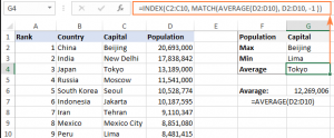
To find the average value in column D and display this value in C:
=ИНДЕКС(С2:С10,ПОИСКПОЗ(СРЗНАЧ(D2:D10),D2:D10,-1))
Depending on how your data is written, the third argument to MATCH() is either 1, 0, or -1:
- if the columns are sorted in ascending order, set 1 (then the formula will calculate the maximum value, which is less than or equal to the average value);
- if the sort is descending, then -1 (the formula will output the minimum value that is greater than or equal to the average);
- if the lookup array contains a value that is exactly equal to the average, then set it to 0.
In our example, the population is sorted in descending order, so we put -1. And the result is Tokyo, since the population value (13,189) is the closest to the average value (000).
VLOOKUP() can also perform such calculations, but only as an array formula: VLOOKUP with AVERAGE, MIN and MAX.
INDEX MATCH and ESND/IFERROR
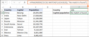
You probably already noticed that if the formula cannot find the desired value, it throws an error # N / A. You can replace the standard error message with something more informative. For example, set the argument in the formula In the XNUMXth:
=ЕСНД(ИНДЕКС(С2:С10,ПОИСКПОЗ(F1,A2:A10,0)),значение не найдено)
With this formula, if you enter data that is not in the table, the form will give you the specified message.
If you want to catch all errors, then except for In the XNUMXth קענען זייַן געוויינט פאַלש:
=IFERROR(INDEX(C2:C10,MATCH(F1,A2:A10,0)), “Something went wrong!”)
But remember that masking errors in this way is not a good idea, because standard errors report violations in the formula.
We hope you found our guide to using the INDEX MATCH() function helpful.