גער נומערן-ווי-טעקסט צו נאָרמאַל נומערן

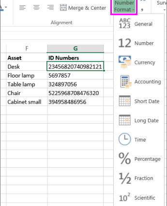
If the text format was set for any cells on the sheet (this could be done by the user or the program when uploading data to Excel), then the numbers entered later into these cells Excel starts to consider as text. Sometimes such cells are marked with a green indicator, which you have most likely seen:

And sometimes such an indicator does not appear (which is much worse).

In general, the appearance of numbers-as-text in your data usually leads to a lot of very unfortunate consequences:

• sorting stops working normally – “pseudo-numbers” are squeezed out, and are not arranged in order as expected:

  
  

• type functions VLOOKUP (VLOOKUP) do not find the required values, because for them the number and the same number-as-text are different:

  
  

• when filtering, pseudo-numbers are selected erroneously
  
• many other Excel functions also stop working properly:
• אאז"ו ו

It is especially funny that the natural desire to simply change the cell format to numeric does not help. Those. you literally select cells, right click on them, select צעל פֿאָרמאַט (פֿאָרמאַט צעלן), change the format to נומעריש (נומער), squeeze OK — and nothing happens! At all!

Perhaps, “this is not a bug, but a feature”, of course, but this does not make it easier for us. So let’s look at several ways to fix the situation – one of them will definitely help you.

Method 1. Green indicator corner

If you see a green indicator corner on a cell with a number in text format, then consider yourself lucky. You can simply select all cells with data and click on the pop-up yellow icon with an exclamation mark, and then select the command גער צו נומער (Convert to number):

All numbers in the selected range will be converted to full numbers.

If there are no green corners at all, then check if they are turned off in your Excel settings (File – Options – Formulas – Numbers formatted as text or preceded by an apostrophe).

Method 2: Re-entry

If there are not many cells, then you can change their format to numeric, and then re-enter the data so that the format change takes effect. The easiest way to do this is by standing on the cell and pressing the keys in sequence F2 (enter edit mode, the cell starts blinking cursor) and then אַרייַן. Also instead of F2 you can simply double-click on the cell with the left mouse button.

It goes without saying that if there are a lot of cells, then this method, of course, will not work.

אופֿן 3. פאָרמולע

You can quickly convert pseudo-numbers to normal ones if you make an additional column with an elementary formula next to the data:

Double minus, in this case, means, in fact, multiplying by -1 twice. A minus by a minus will give a plus and the value in the cell will not change, but the very fact of performing a mathematical operation switches the data format to the numerical one we need.

Of course, instead of multiplying by 1, you can use any other harmless mathematical operation: division by 1 or adding and subtracting zero. The effect will be the same.

אופֿן 4: פּאַפּ ספּעציעלע

This method was used in older versions of Excel, when modern effective managers went under the table  there was no green indicator corner yet in principle (it appeared only in 2003). The algorithm is this:

• enter 1 in any empty cell
• נאָכמאַכן עס
• select cells with numbers in text format and change their format to numeric (nothing will happen)
• right-click on cells with pseudo-numbers and select command פּאַפּ ספּעציעל (פּיסט ספּעציעלע) אָדער נוצן קלאַוויאַטור דורכוועג קטרל + אַלט + V.
• in the window that opens, select the option די וואַלועס (ווערטן) и מערן (מערן)

In fact, we do the same thing as in the previous method – multiplying the contents of the cells by one – but not with formulas, but directly from the buffer.

אופֿן 5. טעקסט דורך שפאלטן

If the pseudonumbers to be converted are also written with incorrect decimal or thousands separators, another approach can be used. Select the source range with data and click the button טעקסט דורך שפאלטן (Text to columns) קוויטל דאַטע (דאַטע). In fact, this tool is designed to divide sticky text into columns, but, in this case, we use it for a different purpose.

Skip the first two steps by clicking on the button ווייַטער (ווייַטער), and on the third, use the button אַדישנאַלי (אַוואַנסירטע). A dialog box will open where you can set the separator characters currently available in our text:

נאָך דריקט אויף ענדיקן Excel will convert our text to normal numbers.

אופֿן 6. מאַקראָו

If you have to do such transformations often, then it makes sense to automate this process with a simple macro. Press Alt+F11 or open a tab דעוועלאָפּער (דעוועלאָפּער) און גיט די וויסואַל באַסיק. In the editor window that appears, add a new module through the menu אַרייַנלייגן - מאָדולע און קאָפּיע די פאלגענדע קאָד דאָרט:

Sub Convert_Text_to_Numbers()      Selection.NumberFormat = "General"      Selection.Value = Selection.Value  End Sub  

Now after selecting the range, you can always open the tab דעוועלאָפּער - מאַקראָס (דעוועלאָפּער - מאַקראָס), select our macro in the list, press the button לויפן (לויפן) – and instantly convert pseudo-numbers into full-fledged ones.

You can also add this macro to your personal macro book for later use in any file.

PS

The same story happens with dates. Some dates may also be recognized by Excel as text, so grouping and sorting will not work. The solutions are the same as for numbers, only the format must be replaced with a date-time instead of a numeric one.

• Dividing sticky text into columns
• Calculations without formulas by special pasting
• Convert text to numbers with the PLEX add-on