ינהאַלט
נעכטן אין די מעראַטאַן 30 עקססעל פאַנגקשאַנז אין 30 טעג we counted the number of columns in the range using the function שפאלטן (NUMBERCOLUMN), and now it’s time for something more in demand.
On the 13th day of the marathon, we will devote to the study of the function יבערשיקן (TRANSP). With this function, you can rotate your data by turning vertical areas into horizontal ones and vice versa. Do you have such a need? Can you do this using a special insert? Can other functions do it?
So, let’s turn to information and examples on the function יבערשיקן (TRANSP). If you have additional information or examples, please share them in the comments.
Function 13: TRANSPOSE
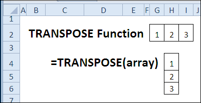
פונקציע יבערשיקן (TRANSPOSE) returns a horizontal range of cells as a vertical range, or vice versa.
How can the TRANSPOSE function be used?
פונקציע יבערשיקן (TRANSP) can change the orientation of the data, as well as work in conjunction with other functions:
- Change the horizontal layout of data to vertical.
- Show the best total wages in recent years.
To change the data orientation without creating links to the original data:
- נוצן פּאַפּ ספּעציעלע (ספּעציעלע פּאַפּ) > יבערזעצונג (טראַנספּאָסע).
Syntax TRANSPOSE (TRANSP)
פונקציע יבערשיקן (TRANSPOSE) has the following syntax:
TRANSPOSE(array)
ТРАНСП(массив)
- מענגע (array) is the array or range of cells to be transposed.
Traps TRANSPOSE (TRANSPOSE)
- פונקציע יבערשיקן (TRANSPOSE) must be entered as an array formula, by pressing Ctrl + Shift + Enter.
- The range that will result from the transformation by the function יבערשיקן (TRANSPOSE) must have the same number of rows and columns as the original range has columns and rows respectively.
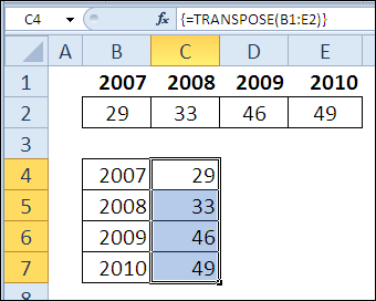
Example 1: Turning Horizontal Data into Vertical Data
If the data is horizontal in an Excel sheet, you can apply the function יבערשיקן (TRANSPOSE) to convert them to a vertical position, but in a different place on the sheet. For example, in the final table of benchmarks, a vertical arrangement would be more convenient. Using the function יבערשיקן (TRANSPOSE), you can reference the original horizontal data without changing its location.
To transpose the horizontal range קסנומקס × קסנומקס into the vertical range קסנומקס × קסנומקס:
- Select 8 cells where you want to place the resulting vertical range. In our example, these will be cells B4:C7.
- Enter the following formula and turn it into an array formula by clicking Ctrl + Shift + Enter.
=TRANSPOSE(B1:E2)
=ТРАНСП(B1:E2)
Curly braces will automatically be added at the beginning and end of the formula to indicate that an array formula has been entered.
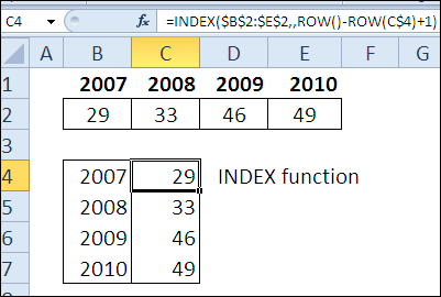
אָנשטאָט יבערשיקן (TRANSPOSE), You can use another function to transform the data, for example, ינדעקס (INDEX). It doesn’t require you to enter an array formula, and you don’t have to select all the cells in the target area when creating the formula.
=INDEX($B$2:$E$2,,ROW()-ROW(C$4)+1)
=ИНДЕКС($B$2:$E$2;;СТРОКА()-СТРОКА(C$4)+1)
Example 2: Change orientation without links
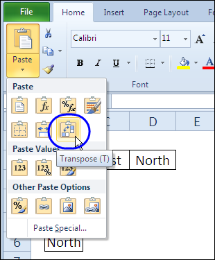
If you just want to change the orientation of your data without keeping a reference to the original data, you can use Paste Special:
- Select source data and copy it.
- Select the top left cell of the area where you want to place the result.
- אויף די אַוואַנסירטע קוויטל היים (Home) click on the command dropdown menu פּאַפּ (אַרייַנלייגן).
- סעלעקטירן יבערזעצונג (טראַנספּאָסע).
- Delete the original data (optional).
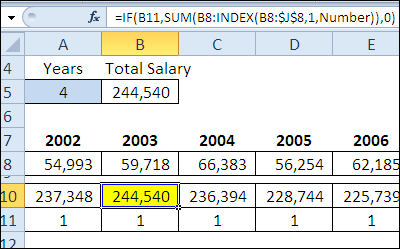
Example 3: Best Total Salary in Past Years
פונקציע יבערשיקן (TRANSP) can be used in combination with other features, such as in this stunning formula. It was posted by Harlan Grove in the Excel News Bloc in a discussion about calculating the best total wage for the past 5 years (in a row!).
=MAX(MMULT(A8:J8, --(ABS(TRANSPOSE(COLUMN(A8:J8))-COLUMN(OFFSET(A8:J8,0,0,1,COLUMNS(A8:J8)-Number+1))-(Number-1)/2)
=МАКС(МУМНОЖ(A8:J8; --(ABS(ТРАНСП(СТОЛБЕЦ(A8:J8))-СТОЛБЕЦ(СМЕЩ(A8:J8;0;0;1;ЧИСЛСТОЛБ(A8:J8)-Number+1))-(Number-1)/2)
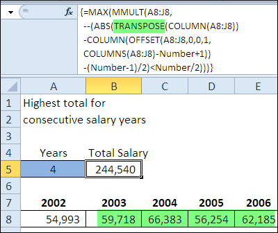
Как можно понять по фигурным скобкам в строке формул – это формула массива. Ячейка A5 названа נומער и в этом примере число 4 введено, как значение для количества лет.
Формула проверяет диапазоны, чтобы увидеть достаточно ли в них последовательных столбцов. Результаты проверки (1 или 0) умножаются на значения ячеек, чтобы получить суммарный объём заработной платы.
Для проверки результата на рисунке ниже в строке под значениями зарплат показаны суммарные значения для каждой стартовой ячейки, при этом максимальное значение выделено жёлтым. Это более долгий путь к тому же результату, что предыдущая формула массива получает в одной ячейке!