ווי צו אַראָפּרעכענען / לייגן אַ פּראָצענט פון אַ נומער אין עקססעל (+ ביישפילן)

The ability to determine the percentage of a number and perform various operations with them is very important in completely different areas of activity – accounting, investments, and even when dining in a restaurant. There is no area of ​​life in which it would not be necessary from time to time to determine the part of the whole.

Excel has a whole set of tools that allow you to perform operations with percentages. Most of them are performed automatically, just enter the formula, and the desired value will be calculated. Very comfortably.

How to work with percentages in Excel

Everyone now knows how to determine percentages. And even if he doesn’t know how, it can always be done using a calculator (although there is hardly anyone like that). On this device, operations with percentages are performed through a special% icon. 

With Excel, this is even easier than on your own. But before you draw up formulas and perform some operations with them, you need to remember the basics of school.

A percentage is a hundredth of a number. To determine it, you need to divide the part by the integer value and multiply the result by 100. 

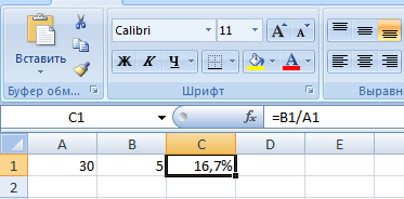
Let’s say you are a warehouse manager. 30 units of products were delivered to you. On the first day, only 5 of them were realized. So what percentage of the product was actually sold?

We understand that 5 is a fraction and 30 is an integer. Next, you just need to insert the appropriate numbers into the formula described above, after which we get the result of 16,7%.

Adding a percentage to a number in the standard way is somewhat more difficult, since this operation is performed in several steps.

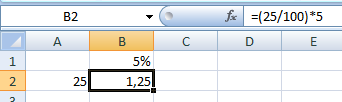
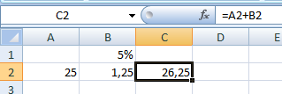
First you need to determine 5%, and then add this value to the number. For example, if you add 5% to 25, the final result will be 26,5.

Now, after we know the rules for working with percentages in real life, it is not so difficult to understand how it works in Excel.

Calculating percentage of a number in Excel

To do this, you can use several methods.

Let’s imagine that we have such a table. The first cell horizontally is the total quantity of goods, and the second, respectively, How long of it was sold. In the third, we will perform a mathematical operation.

Now let’s take a closer look at this picture. Don’t see anything surprising? The formula bar shows a simple division of a part of a whole, the percentage is displayed, but we did not multiply the result by 100. Why is this happening?

The fact is that each cell in Excel can have its own format. In the case of C1, a percentage is used. That is, the program automatically multiplies the result by 100, and the % sign is added to the result. If there is such a need, the user can determine how many decimal places should be displayed in the resulting result. 

Now let’s determine what number is five percent of the number 25. To do this, you must first multiply these values, and then divide them by 100. The result is visible in the screenshot.

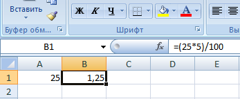
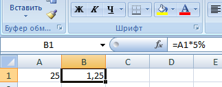
Well, or the second option is to divide the integer by one hundred, and then multiply by 5. The result will not change from this. 

This task can be realized in another way. To do this, you need to find the% sign on the keyboard (to add it, you need to simultaneously press the number 5 with the Shift key).

And now let’s check in practice how you can use the knowledge gained.

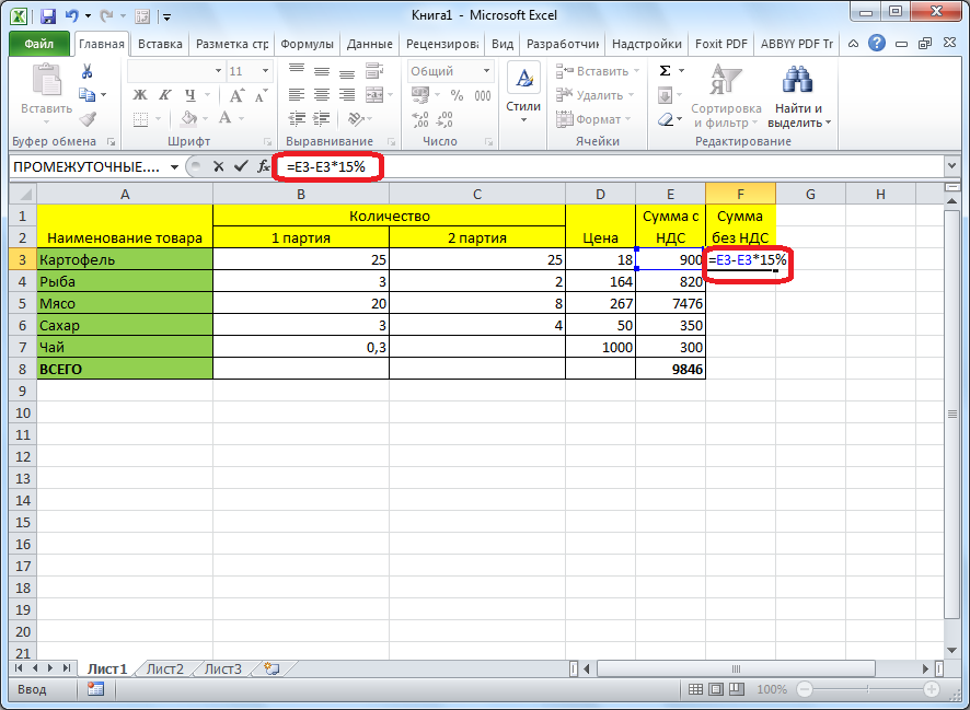
Suppose we have a table listing commodity items, their cost, and we also know the VAT rate (suppose it is 18%). Accordingly, in the third column it is necessary to record the amount of tax.

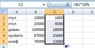
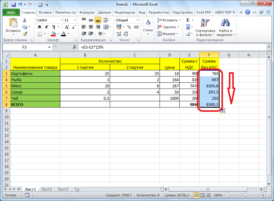
After the product price has been multiplied by 18%, you need to use the auto-complete marker to write this formula in each cell of the column. To do this, you need to click on the box located in the lower right corner and drag it down to the desired number of cells. 

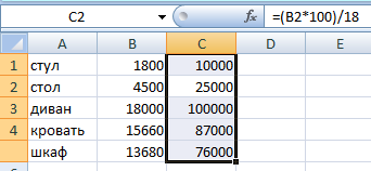
After we have received the tax amount, it is necessary to determine How long the user will have to pay in the end.

די פאָרמולע איז ווי גייט:

=(B1*100)/18

After we applied it, we get such a result in the table.

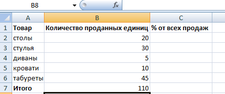
We know how many items were sold as a whole and individually. We now need to understand what percentage of the total sales is for each unit.

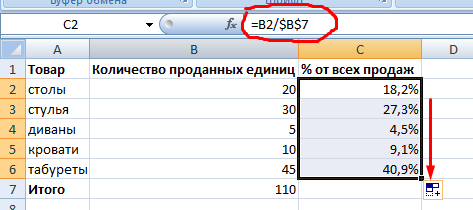
The formula does not change. You need to divide the share by an integer value, and multiply the result by 100. But in this case, you need to make the link absolute. To do this, precede the row number and column designation with a dollar sign $. You will get the following result.

Adding a percentage to a number in Excel

To do this, you need to follow two steps:

1. Determine the percentage of a number. In our case it is 1,25.
   

   

2. The resulting result is added to the integer. In our example, the result will be 26,5. That is, the sequence of actions is the same as with standard calculations, just all calculations are performed inside Excel.
   

   

And on this table, we directly add the values. Let’s not focus on the intermediate action.

Initially, we have a table like this.

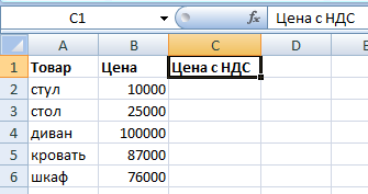
We know that in our example the VAT rate is set at 18 percent. Therefore, to determine the total amount of goods with VAT, you must first determine the amount of tax, and then add it to the price.

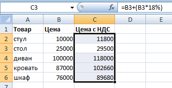
It is important to remember to write the parentheses, as they tell the program in which order to perform mathematical operations.

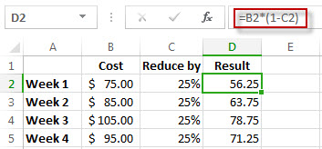
To decrease a number by a certain percentage, the formula is approximately the same, except that instead of adding, a subtraction operation is performed.

Calculate Percentage Difference in Excel

The difference is a measure expressing the degree of price change, expressed in a certain unit. In our case, these are percentages. 

Let’s not think about Excel first, but consider the situation as a whole. Suppose tables cost 100 rubles a month ago, and now they cost 150 rubles. 

In this case, the following formula must be applied to determine to what extent this value has been changed.

Percent difference = (new data – old data) / old data * 100%.

In our case, the price increased by 50%.

subtraction percentage in excel

And now we will describe how to do the same in Excel. Here is a screenshot for clarity. Pay attention to the formula bar.

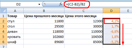
It is important to set the percentage format so that the values ​​are displayed correctly.

If you need to calculate by what percentage the price has changed compared to the one indicated in the previous line, you need to use this formula (pay attention to the screenshot).

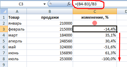
אין אַלגעמיין, עס קוקט ווי דאָס: (next value – previous value) / previous value.

Since the specificity of the data does not provide for the possibility of introducing a percentage change in a row, it can simply be skipped. 

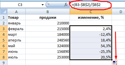
Sometimes it may be necessary to make a comparison with January. To do this, you need to turn the link into an absolute one, and then simply use the autocomplete marker when necessary.

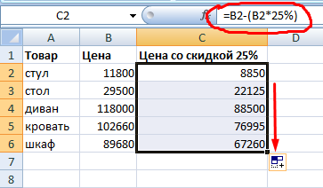
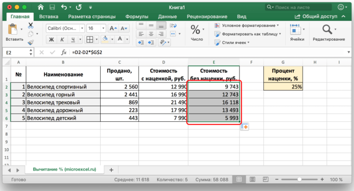
Subtracting percentages from a completed excel spreadsheet

But what if the information is already entered in the table? In this case, you must first place the cursor on the top empty cell and put the = sign. After that, click on the cell that contains the value from which you want to determine the percentage. Next, press – (to perform the subtraction operation) and click on the same cell). Then we press the star icon (denoting the multiplication operation in Excel) and type the number of percentages that need to be subtracted from this number. After that, simply write the percent sign and confirm the entry of the formula with the Enter key.

The result will appear in the same cell where the formula was written.

To copy it further down the column and perform a similar operation with respect to other rows, you must use the autocomplete marker as described above. That is, drag the cell in the lower right corner to the required number of cells down. After that, in each cell you will get the result of subtracting a certain percentage from a larger number.

Subtraction of interest in a table with a fixed percentage

Suppose we have such a table.

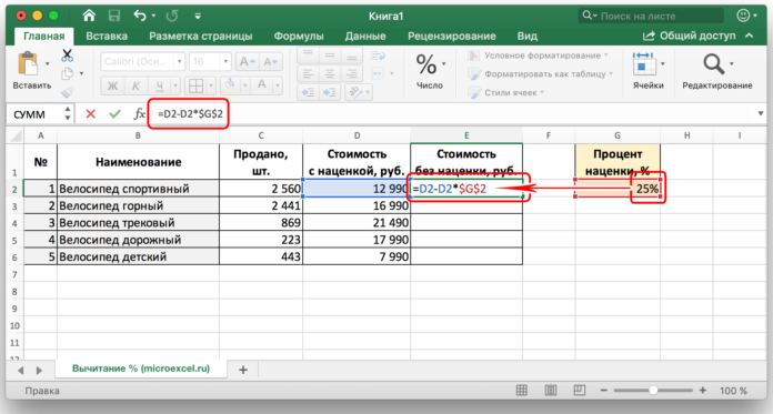
In it, one of the cells contains a percentage that does not change in all calculations in all cells of this column. The formula that is used in this situation is visible in the screenshot above (cell G2 just contains such a fixed percentage).

The reference sign to the absolute address of a cell can be specified either manually (by simply entering it before the address of a row or column), or by clicking on the cell and pressing the F4 key. 

This will fix the link so that it does not change when copied to other cells. After pressing the Enter key, we get the finished calculated result.

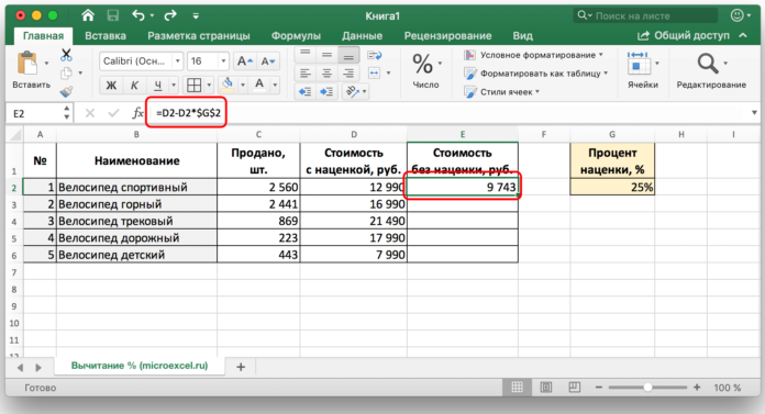
After that, in the same way as in the examples above, you can use the autocomplete marker to stretch the formula to all the cells in the column.

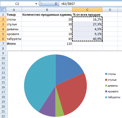
Create a percentage chart in Excel

In some situations, you may want to create a percentage chart. This can be done in several ways. The first one is to create a column that will list the percentages to be used as the data source. In our case, this is a percentage of all sales.

Further, the sequence of actions is as follows:

1. Select a table with information. In our case, this is a list of percentages.
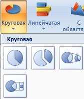
2. Go to the “Insert” – “Diagram” tab. We are going to create a pie chart, so this is the type we choose.
   

   

3. Next, you will be prompted to choose the appearance of the future diagram. After we select it, it automatically appears.
   

   

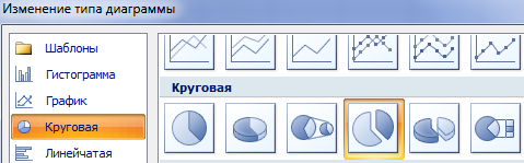
Then you can configure it through the special tab “Working with diagrams” – “Designer”. There you can choose many different types of settings:

1. Changing the chart type. If you click on the corresponding button, you will be able to set the chart type.
   

   

2. Swap rows and columns. 
3. Change the data that is used in the chart. A very useful feature if the percentage list needs to be changed. For example, you can copy sales information from last month, replace it with another column with new percentages, and then change the data for the chart to the current one.
4. Edit chart design. 
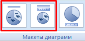
5. Edit templates and layouts. 

The last option is of particular interest to us, because it is through it that you can set the percentage format. Just in the list of layouts that was offered by Excel, we find the option in which the percentage icons are drawn in the sectors.

You can also display data in percentage format in another way. To do this, click on the existing pie chart, go to the “Layout” tab and find the “Data Labels” option there.

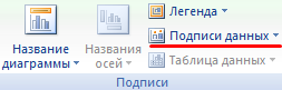
A list of functions will open in which you need to select the location of the signatures.

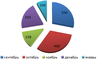
After we do this, the percentage image will appear on the chart.

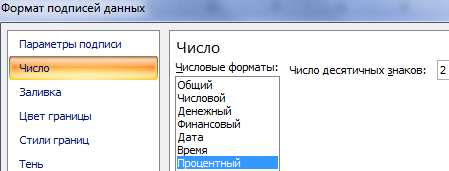
If you right-click on one of them, then through the “Data Label Format” menu, you can more flexibly configure the labels. In our case, we are interested in including shares in signatures, because this item must be selected to confirm the percentage format.

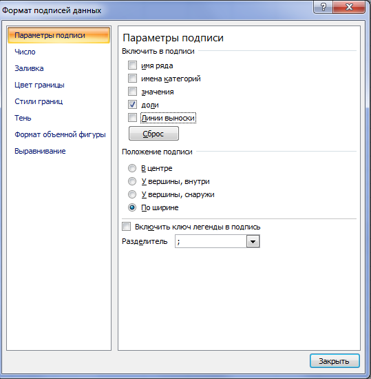
And the percentage format itself is set in the “Number” menu, which can be opened through the panel located on the left side of the dialog box.

As you can see, working with percentages in Excel does not require special skills. You just need to learn a few tricks to perform even complex tasks with ease and elegance. Of course, these are not all the functions available to the Excel user, since percentages can also be controlled by other methods, for example, through a macro. But this is already a really advanced level, requiring knowledge of more complex topics. Therefore, it is logical to leave the work with percentages through macros for later. 

Percentages are very convenient to use in a number of formulas, each of which can be adapted to the needs of a particular user.