ווי צו ראָונד אַ נומער אין עקססעל. נומער פֿאָרמאַט דורך די קאָנטעקסט מעניו, באַשטעטיקן די פארלאנגט אַקיעראַסי, אַרויסווייַזן סעטטינגס

The spreadsheet Excel has a wide functionality that allows you to perform a variety of manipulations with numerical information. It often happens that when carrying out various actions, fractional values ​​are rounded off. This is a very useful feature, since most of the work in the program does not require accurate results. However, there are such calculations where it is necessary to preserve the accuracy of the result, without the use of rounding. There are many ways to work with rounding numbers. Let’s look at everything in more detail.

How numbers are stored in Excel and displayed on the screen

The spreadsheet process works on two types of numerical information: approximate and exact. A person working in a spreadsheet editor can choose the method for displaying a numerical value, but in Excel itself, the data is in the exact form – up to fifteen characters after the decimal point. In other words, if the display shows data up to two decimal places, then the spreadsheet will refer to a more accurate record in memory during calculations.

You can customize the display of numerical information on the display. The rounding procedure is carried out according to the following rules: indicators from zero to four inclusive are rounded down, and from five to nine – to a larger one.

Features of rounding Excel numbers

Let us examine in detail several methods for rounding numerical information.

Rounding with Ribbon Buttons

Consider an easy rounding editing method. Detailed instructions look like this:

1. We select a cell or a range of cells.
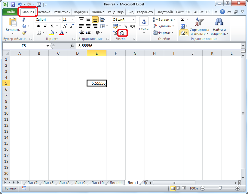
2. We move to the “Home” section and in the “Number” command block, click LMB on the “Decrease bit depth” or “Increase bit depth” element. It is worth noting that only selected numeric data will be rounded, but up to fifteen digits of the number are used for calculations.
3. The increase in characters by one after the comma occurs after clicking on the element “Increase bit depth”.

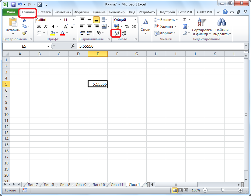
4. Decreasing characters by one is done after clicking on the “Decrease bit depth” element.

Rounding Through Cell Format

Using the box called “Cell Format”, it is also possible to implement rounding editing. Detailed instructions look like this:

1. We select a cell or range.
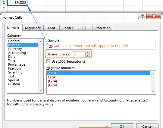
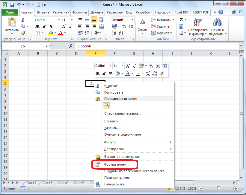
2. Click RMB on the selected area. A special context menu has opened. Here we find an element called “Format Cells …” and click LMB.

3. The Format Cells window appears. Go to the “Number” subsection. We pay attention to the column “Numeric formats:” and set the indicator “Numeric”. If you select a different format, the program will not be able to implement rounding numbers.. In the center of the window next to “Number of decimal places:” we set the number of characters that we plan to see during the procedure.

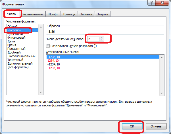
4. At the end, click on the “OK” element to confirm all the changes made.

Set calculation accuracy

In the methods described above, the parameters set had an impact only on the external output of numerical information, and when performing calculations, more accurate values ​​were used (up to the fifteenth character). Let’s talk in more detail about how to edit the accuracy of calculations. Detailed instructions look like this:

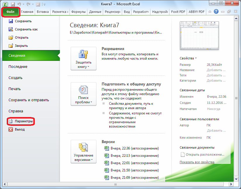
1. Go to the “File” section, and then on the left side of the new window we find an element called “Parameters” and click on it with LMB.

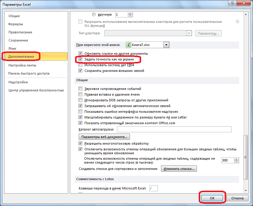
2. A box called “Excel Options” appears on the display. We move to “Advanced”. We find the block of commands “When recalculating this book.” It is worth noting that the changes made will apply to the entire book. Put a checkmark next to the inscription “Set accuracy as on the screen.” Finally, click on the “OK” element to confirm all the changes made.

3. Ready! Now, when calculating information, the output value of numerical data on the display will be taken into account, and not the one that is stored in the memory of the spreadsheet processor. Setting the displayed numerical values ​​is done by any of the 2 methods described above.

Application of functions

ופמערקזאַמקייַט! If the user wants to edit the rounding when calculating relative to one or several cells, but does not plan to reduce the accuracy of calculations in the entire workbook, then he should use the capabilities of the ROUND operator.

This function has several uses, including in combination with other operators. In the main operators, rounding is done:

• “ROUNDDOWN” – to the nearest number down in modulus;
• “ROUNDUP” – up to the closest value up in the modulo;
• “OKRVUP” – with the specified accuracy up the modulo;
• “OTBR” – until the moment when the number becomes an integer type;
• “ROUND” – up to a specified number of decimal characters in accordance with accepted rounding standards;
• “OKRVNIZ” – with the specified accuracy down the modulo;
• “EVEN” – to the nearest even value;
• “OKRUGLT” – with the specified accuracy;
• “ODD” – to the nearest odd value.

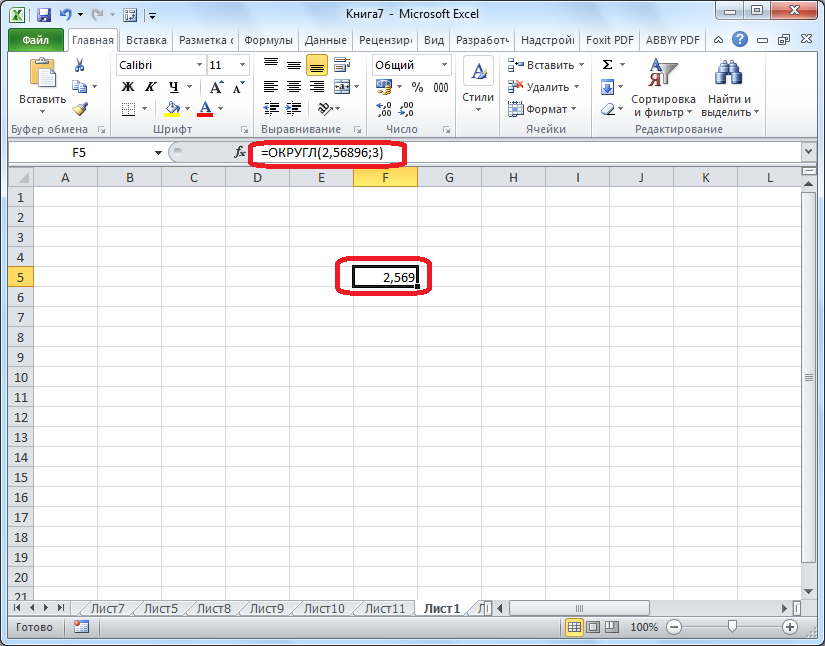
The ROUNDDOWN, ROUND, and ROUNDUP operators have the following general form: =Name of the operator (number;number_digits). Suppose the user wants to perform a rounding procedure for the value 2,56896 to 3 decimal places, then he needs to enter “=ROUND(2,56896;3)”. Ultimately, he will receive:

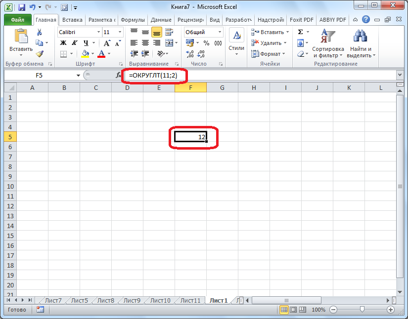
Operators “ROUNDDOWN”, “ROUND”, and “ROUNDUP” have the following general form: =Name of operator(number,precision). If the user wants to round the value 11 to the nearest multiple of two, then he needs to enter “=ROUND(11;2)”. Ultimately, he will receive:

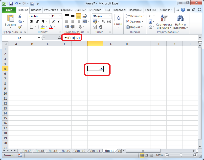
The operators “ODD”, “SELECT”, and “EVEN” have the following general form:  =Name of the operator (number). For example, when rounding the value 17 to the nearest even value, he needs to enter «=THURS(17)». Ultimately, he will receive:

Worth noticing! The operator can be entered in the line of functions or in the cell itself. Before writing a function into a cell, it must be selected in advance with the help of LMB.

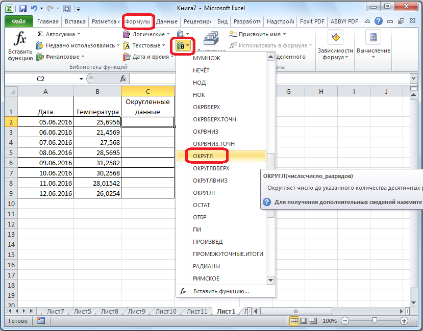
The spreadsheet also has another operator input method that allows you to perform the procedure for rounding numerical information. It’s great for when you have a table of numbers that need to be turned into rounded values ​​in another column. Detailed instructions look like this:

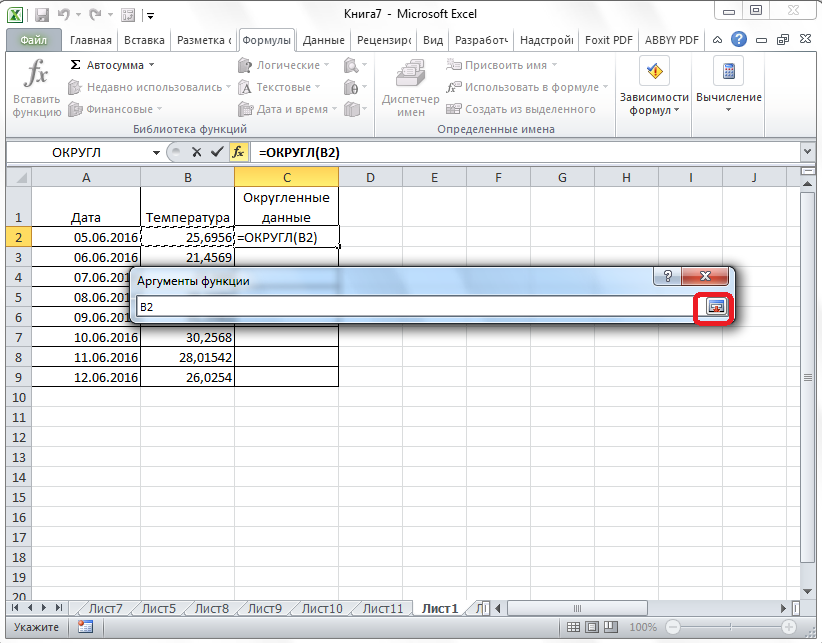
1. We move to the “Formulas” section. Here we find the element “Math” and click on it with LMB. A long list has opened, in which we select an operator called “ROUND”.

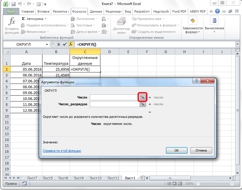
2. A dialog box called “Function Arguments” appeared on the display. The line “Number” can be filled in with information yourself by manual input. An alternative option that allows you to automatically round all information is to click LMB on the icon located to the right of the field for writing an argument.

3. After clicking on this icon, the “Function Arguments” window collapsed. We click LMB on the uppermost field of the column, the information in which we plan to round. The indicator appeared in the arguments box. We click LMB on the icon located to the right of the value that appears.

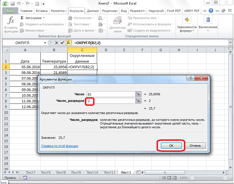
4. The screen again displayed a window called “Function Arguments”. In the line “Number of digits” we drive in the bit depth to which it is necessary to reduce the fractions. Finally, click on the “OK” item to confirm all the changes made.

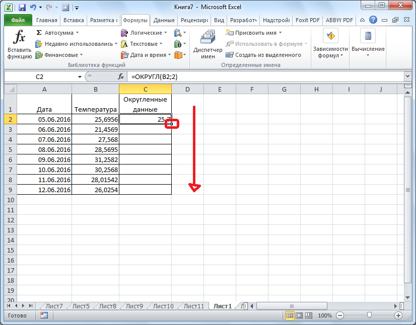
5. The numeric value has been rounded up. Now we need to perform the rounding procedure for all other cells in this column. To do this, move the mouse pointer to the lower right corner of the field with the displayed result, and then, by holding the LMB, stretch the formula to the end of the table.

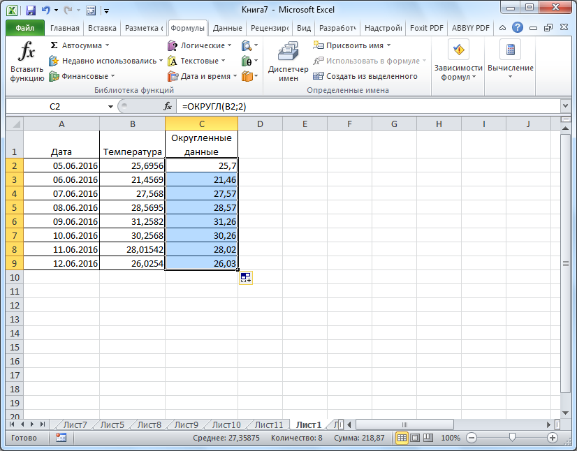
6. Ready! We have implemented a rounding procedure for all cells in this column.

How to round up and down in Excel

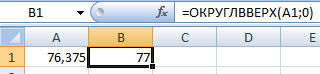
Let’s take a closer look at the ROUNDUP operator. The 1st argument is filled in as follows: the address of the cell is entered with numeric information. Filling in the 2nd argument has the following rules: entering the value “0” means rounding the decimal fraction to an integer part, entering the value “1” means that after the implementation of the rounding procedure there will be one character after the decimal point, etc. Enter the following value in the line for entering formulas: = ROUNDUP (A1). Finally we get:

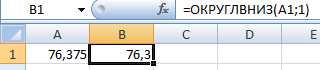
Now let’s look at an example of using the ROUNDDOWN operator. Enter the following value in the line for entering formulas: =ROUNDSAR(A1).Finally we get:

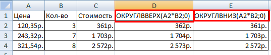
It is worth noting that the operators “ROUNDDOWN” and “ROUNDUP” are additionally used to implement the procedure for rounding the difference, multiplication, etc.

Example of use:

How to round to whole number in Excel?

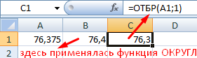
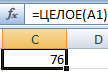
The “SELECT” operator allows you to implement rounding to an integer and discard characters after the decimal point. For an example, consider this image:

A special spreadsheet function called “INT” allows you to return an integer value. There is only one argument – “Number”. You can enter either numeric data or cell coordinates. Example:

The main disadvantage of the operator is that rounding is implemented only down.

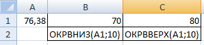
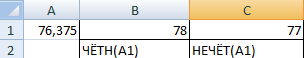
To round numerical information to integer values, it is necessary to use the previously considered operators “ROUNDDOWN”, “EVEN”, “ROUNDUP” and “ODD”. Two examples of using these operators to implement rounding to an integer type:

פארוואס טוט עקססעל קייַלעכיק גרויס נומערן?

If the program element contains a huge value, for example 73753956389257687, then it will take the following form: 7,37539E+16. This is because the field has a “General” view. In order to get rid of this type of output of long values, you need to edit the field format and change the type to Numeric. The key combination “CTRL + SHIFT + 1” will allow you to perform the editing procedure. After making the settings, the number will take the correct form of display.

סאָף

From the article, we found out that in Excel there are 2 main methods for rounding the visible display of numerical information: using the button on the toolbar, as well as editing cell format settings. Additionally, you can implement editing the rounding of the calculated information. There are also several options for this: editing document parameters, as well as using mathematical operators. Each user will be able to choose for himself the most optimal method suitable for his specific goals and objectives.