ינהאַלט
This little tutorial explains how to make a function VPR (VLOOKUP) case-sensitive, shows several other formulas that Excel can search in a case-sensitive manner, and points out the strengths and weaknesses of each function.
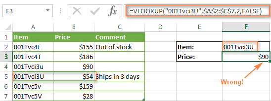
I guess every Excel user knows what function performs vertical search. That’s right, it’s a function VPR. However, few people know that VPR is not case sensitive, i.e. the lower and upper case characters are identical for it.
Here is a quick example demonstrating the inability VPR recognize register. Suppose in a cell A1 contains the value “bill” and the cell A2 – “Bill”, formula:
=VLOOKUP("Bill",A1:A10,2)
=ВПР("Bill";A1:A10;2)
… will stop its search on “bill” since that value comes first in the list, and extract the value from the cell B1.
Later in this article, I’ll show you how to do VPR case sensitive. In addition, we will learn a few more functions that can perform case-sensitive searches in Excel.
We’ll start with the simplest – VIEW (LOOKUP) and SUMPRODUCT (SUMPRODUCT), which, unfortunately, have several significant limitations. Next, we will take a closer look at the slightly more complex formula אינדעקס + גלייַכן (INDEX+MATCH), which works flawlessly in any situation and with any dataset.
VLOOKUP function is case sensitive
As you already know, the usual function VPR is case insensitive. However, there is a way to make it case sensitive. To do this, you need to add an auxiliary column to the table, as shown in the following example.
Suppose in a column B there are product identifiers (Item) and you want to extract the price of the product and the corresponding comment from the columns C и D. The problem is that identifiers contain both lowercase and uppercase characters. For example, cell values B4 (001Tvci3u) and B5 (001Tvci3U) differ only in the case of the last character, u и U ריספּעקטיוולי.
As you can imagine, the usual search formula
=VLOOKUP("001Tvci3U",$A$2:$C$7,2,FALSE)
=ВПР("001Tvci3U";$A$2:$C$7;2;ЛОЖЬ)
וועט צוריקקומען $ קסנומקס, since the value 001Tvci3u is in the search range earlier than 001Tvci3U. But that’s not what we need, is it?
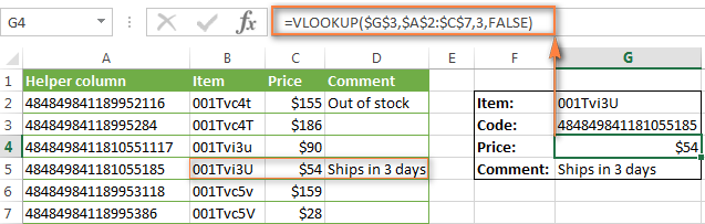
To search with a function VPR in Excel case sensitive, you will have to add a helper column and fill its cells with the following formula (where B is the lookup column):
=CODE(MID(B2,1,1)) & CODE(MID(B2,2,1)) & CODE(MID(B2,3,1)) & CODE(MID(B2,4,1)) & CODE(MID(B2,5,1)) & CODE(MID(B2,6,1)) & CODE(MID(B2,7,1)) & CODE(MID(B2,8,1)) & IFERROR(CODE(MID(B2,9,1)),"")
=КОДСИМВ(ПСТР(B2;1;1)) & КОДСИМВ(ПСТР(B2;2;1)) & КОДСИМВ(ПСТР(B2;3;1)) & КОДСИМВ(ПСТР(B2;4;1)) & КОДСИМВ(ПСТР(B2;5;1)) & КОДСИМВ(ПСТР(B2;6;1)) & КОДСИМВ(ПСТР(B2;7;1)) & КОДСИМВ(ПСТР(B2;8;1)) & ЕСЛИОШИБКА(КОДСИМВ(ПСТР(B2;9;1));"")
This formula breaks the desired value into separate characters, replaces each character with its code (for example, instead of A at 65, instead a code 97) and then combines these codes into a unique string of numbers.
After that, we use a simple function VPR for case sensitive search:
=VLOOKUP($G$3,$A$2:$C$8,3,FALSE)
=ВПР($G$3;$A$2:$C$8;3;ЛОЖЬ)
Proper operation of the function VPR case-sensitive depends on two factors:
- The helper column must be the leftmost column in the viewable range.
- The value you are looking for must contain a character code instead of the real value.
How to use the CODE function correctly
The formula inserted into the cells of the auxiliary column assumes that all of your search values have the same number of characters. If not, then you need to know the smallest and largest numbers and add as many features פאַלש (IFERROR) how many characters is the difference between the shortest and longest searched value.
For example, if the shortest search value is 3 characters and the longest is 5 characters, use this formula:
=CODE(MID(B2,1,1)) & CODE(MID(B2,2,1)) & CODE(MID(B2,3,1)) & IFERROR(CODE(MID(B2,3,1)),"") & IFERROR(CODE(MID(B2,4,1)),"")
=КОДСИМВ(ПСТР(B2;1;1)) & КОДСИМВ(ПСТР(B2;2;1)) & КОДСИМВ(ПСТР(B2;3;1)) & ЕСЛИОШИБКА(КОДСИМВ(ПСТР(B2;3;1));"") & ЕСЛИОШИБКА(КОДСИМВ(ПСТР(B2;4;1));"")
פֿאַר פֿונקציע PSTR (MID) You provide the following arguments:
- 1st argument – טעקסט (text) is the text or cell reference containing the characters to be extracted (in our case it is B2)
- 2st argument – start_num (start_position) is the position of the first of those characters to be extracted. you enter 1 in the first function PSTR, 2 – in the second function PSTR אאז"ו ו
- 3st argument – num_chars (number_of_characters) – Specifies the number of characters to extract from the text. Since we only need 1 character all the time, in all functions we write 1.
לימיטיישאַנז: פונקציע VPR is not the best solution for case-sensitive searches in Excel. First, the addition of an auxiliary column is required. Secondly, the formula does a good job only if the data is homogeneous, or the exact number of characters in the searched values is known. If this is not your case, it is better to use one of the solutions that we show below.
LOOKUP function for case sensitive search
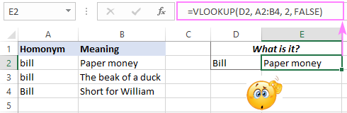
פונקציע VIEW (LOOKUP) related VPR, however its syntax allows for case-sensitive searches without adding an auxiliary column. To do this, use VIEW קאַמביינד מיט די פֿונקציע EXACT (EXACT).
If we take the data from the previous example (without an auxiliary column), then the following formula will cope with the task:
=LOOKUP(TRUE,EXACT($A$2:$A$7,$F$2),$B$2:$B$7)
=ПРОСМОТР(ИСТИНА;СОВПАД($A$2:$A$7;$F$2);$B$2:$B$7)
Formula searches in range A2: אַקסנומקס exact match with cell value F2 case sensitive and returns the value from column B of the same row.
ווי VPRפונקציאָנירן VIEW works equally with text and numeric values, as you can see in the screenshot below:
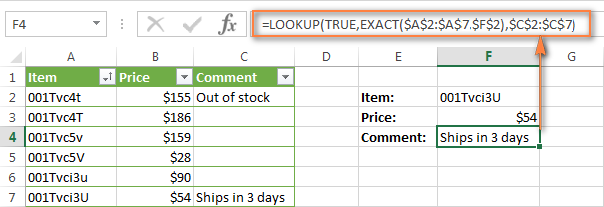
וויכטיק! In order for the function VIEW worked correctly, the values in the lookup column should be sorted in ascending order, i.e. from smallest to largest.
Let me briefly explain how the function works EXACT in the formula shown above, as this is the key point.
פונקציע EXACT compares the two text values in the 1st and 2nd arguments and returns TRUE if they are exactly the same, or FALSE if they are not. It is important for us that the function EXACT case sensitive.
Let’s see how our formula works VIEW+EXACT:
=LOOKUP(TRUE,EXACT($A$2:$A$7,$F$2),$B$2:$B$7)
=ПРОСМОТР(ИСТИНА;СОВПАД($A$2:$A$7;$F$2);$B$2:$B$7)
- פונקציע EXACT compares cell value F2 with all elements in a column A (A2:A7). Returns TRUE if an exact match is found, otherwise FALSE.
- Since you give the first function argument VIEW value TRUE, it extracts the corresponding value from the specified column (in our case, column B) only if an exact match is found, case sensitive.
I hope this explanation was clear and now you understand the main idea. If so, then you will not have any difficulties with other functions that we will analyze further, because. they all work on the same principle.
לימיטיישאַנז: The data in the lookup column must be sorted in ascending order.
SUMPRODUCT – finds text values, case sensitive, but returns only numbers
As you already understood from the title, SUMPRODUCT (SUMPRODUCT) is another Excel function that will help you do a case-sensitive search, but will only return numeric values. If this option does not suit you, then you can immediately proceed to the bundle אינדעקס + גלייַכן, which gives a solution for any case and for any data types.
First, let me briefly explain the syntax of this function, this will help you better understand the case-sensitive formula that follows.
פונקציע SUMPRODUCT multiplies the elements of the given arrays and returns the sum of the results. The syntax looks like this:
SUMPRODUCT(array1,[array2],[array3],...)
СУММПРОИЗВ(массив1;[массив2];[массив3];…)
Since we need a case-sensitive search, we use the function EXACT (EXACT) from the previous example as one of the multipliers:
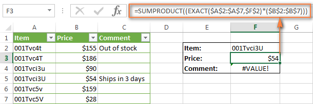
=SUMPRODUCT((EXACT($A$2:$A$7,$F$2)*($B$2:$B$7)))
=СУММПРОИЗВ((СОВПАД($A$2:$A$7;$F$2)*($B$2:$B$7)))
ווי איר געדענקט EXACT compares cell value F2 with all elements in a column A. Returns TRUE if an exact match is found, otherwise FALSE. In mathematical operations, Excel takes TRUE as 1, and FALSE for 0ווייַטער SUMPRODUCT multiplies these numbers and sums the results.
Zeros are not counted because when multiplied they always give 0. Let’s take a closer look at what happens when an exact match in a column A found and returned 1… פֿונקציע SUMPRODUCT multiplies the number in the column B on 1 and returns the result – exactly the same number! This is because the results of the other products are zero, and they do not affect the resulting sum.
צום באַדויערן די פֿונקציע SUMPRODUCT cannot work with text values and dates as they cannot be multiplied. In this case, you will receive an error message # וואָלו! (#VALUE!) as in a cell F4 in the picture below:
לימיטיישאַנז: Returns only numeric values.
INDEX + MATCH – case-sensitive search for any data type
Finally, we are close to an unlimited and case-sensitive search formula that works with any data set.
This example comes last, not because the best is left for dessert, but because the knowledge gained from the previous examples will help you understand the case-sensitive formula better and faster. אינדעקס + גלייַכן (INDEX+MATCH).
As you probably guessed, the combination of functions מער יקספּאָוזד и ינדעקס used in Excel as a more flexible and powerful alternative for VPR. The article Using INDEX and MATCH instead of VLOOKUP will perfectly explain how these functions work together.
I’ll just recap the key points:
- פונקציע מער יקספּאָוזד (MATCH) searches for a value in a given range and returns its relative position, that is, the row and/or column number;
- Next, the function ינדעקס (INDEX) returns a value from a specified column and/or row.
To formula אינדעקס + גלייַכן could search case-sensitively, you only need to add one function to it. It’s not hard to guess what it is again EXACT (EXACT):
=INDEX($B$2:$B$7,MATCH(TRUE,EXACT($A$2:$A$7,$F$2),0))
=ИНДЕКС($B$2:$B$7;ПОИСКПОЗ(ИСТИНА;СОВПАД($A$2:$A$7;$F$2);0))
In this formula EXACT works in the same way as in conjunction with the function VIEW, and gives the same result:
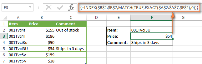
Note that the formula אינדעקס + גלייַכן enclosed in curly braces is an array formula and you must complete it by pressing Ctrl + Shift + Enter.
Why is INDEX+MATCH the best solution for case-sensitive search?
The main advantages of the bundle ינדעקס и מער יקספּאָוזד:
- Does not require adding an auxiliary column, unlike VPR.
- Does not require the search column to be sorted, unlike VIEW.
- Works with all types of data – numbers, text and dates.
This formula seems perfect, doesn’t it? Actually, it is not. And that’s why.
Assume that the cell in the return value column associated with the lookup value is empty. What result will the formula return? No? Let’s see what the formula actually returns:
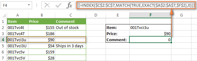
Oops, the formula returns zero! This may not be a big problem if you are working with pure text values. However, if the table contains numbers, including “real” zeros, this becomes a problem.
In fact, all the other lookup formulas (VLOOKUP, LOOKUP, and SUMPRODUCT) we discussed earlier behave the same way. But you want the perfect formula, right?
To make a formula case sensitive אינדעקס + גלייַכן perfect, put it in a function IF (IF) that will test a cell with a return value and return an empty result if it is empty:
=IF(INDIRECT("B"&(1+MATCH(TRUE,EXACT($A$2:$A$7,$G$2),0)))<>"",INDEX($B$2:$B$7, MATCH(TRUE,EXACT($A$2:$A$7,$G$2),0)),"")
=ЕСЛИ(ДВССЫЛ("B"&(1+ПОИСКПОЗ(ИСТИНА;СОВПАД($A$2:$A$7;$G$2);0)))<>"";ИНДЕКС($B$2:$B$7; ПОИСКПОЗ(ИСТИНА;СОВПАД($A$2:$A$7;$G$2);0));"")
אין דעם פאָרמולע:
- B is a column with return values
- 1+ is a number that turns the relative position of the cell returned by the function מער יקספּאָוזד, to the real address of the cell. For example, in our function מער יקספּאָוזד search array given A2: אַקסנומקס, that is, the relative position of the cell A2 וועל 1, because it’s the first one in the array. But the actual position of the cell A2 in the column is 2, so we add 1to make up the difference and to have the function ינדירעקט (INDIRECT) retrieved the value from the desired cell.
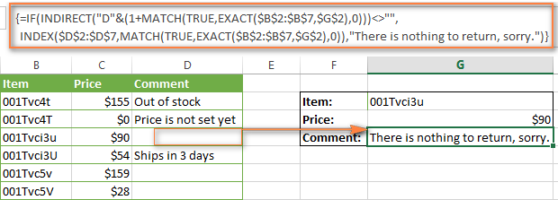
The pictures below show the corrected case-sensitive formula אינדעקס + גלייַכן In action. It returns an empty result if the returned cell is empty.
I rewrote the formula into columns B:Dto fit the formula bar on the screenshot.
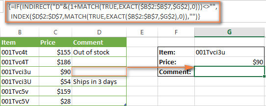
פאָרמולע קערט 0if the returned cell contains zero.
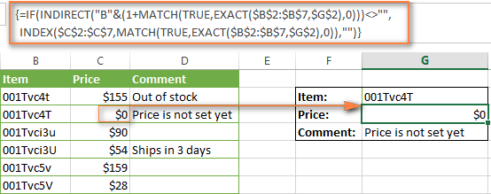
If you want the link ינדעקס и מער יקספּאָוזד displayed some message when the return value is empty, you can write it in the last quotes (“”) of the formula, for example, like this:
=IF(INDIRECT("D"&(1+MATCH(TRUE,EXACT($B$2:$B$7,$G$2),0)))<>"",INDEX($D$2:$D$7, MATCH(TRUE,EXACT($B$2:$B$7,$G$2),0)),"There is nothing to return, sorry.")
=ЕСЛИ(ДВССЫЛ("D"&(1+ПОИСКПОЗ(ИСТИНА;СОВПАД($B$2:$B$7;$G$2);0)))<>"";ИНДЕКС($D$2:$D$7; ПОИСКПОЗ(ИСТИНА;СОВПАД($B$2:$B$7;$G$2);0));"There is nothing to return, sorry.")