30 עקססעל פאַנגקשאַנז אין 30 טעג: קאָד

Congratulations! You made it to the end of the first week of the marathon 30 עקססעל פאַנגקשאַנז אין 30 טעג, having studied the function yesterday פאַרפעסטיקט (FIXED). Today we’re going to relax a bit and take a look at a function that doesn’t have many use cases – the function קאָד (CODE). It can work together with other functions in long and complex formulas, but today we will focus on what it can do on its own in the simplest cases.

So, let’s deal with the reference information on the function קאָד (CODE) and consider the options for its use in Excel. If you have tips or examples of use, please share them in the comments.

Function 07: CODE

פונקציע קאָד (CODE) returns the numeric code of the first character of a text string. For Windows, this will be the code from the table ANSI, and for Macintosh – the code from the symbol table מאַסינטאָש.

How can you use the CODE function?

פונקציע קאָד (CODESYMB) allows you to find the answer to the following questions:

• What is the hidden character at the end of the imported text?
• How can I enter a special character in a cell?

Syntax CODE

פונקציע קאָד (CODE) has the following syntax:

CODE(text)

КОДСИМВ(текст)

• טעקסט (text) is a text string whose first character code you want to get.

Traps CODE (CODE)

The results returned by the function may vary on different operating systems. The ASCII character codes (32 to 126) mostly correspond to the characters on your keyboard. However, the characters for higher numbers (from 129 to 254) may differ.

Example 1: Get hidden character code

Text copied from a website sometimes contains hidden characters. Function קאָד (CODE) can be used to determine what these characters are. For example, cell B3 contains a text string that contains the word “פּראָבע‘ is 4 characters in total. In cell C3, the function LEN (DLSTR) calculated that there are 3 characters in cell B5.

To determine the code of the last character, you can use the function רעכט (RIGHT) to extract the last character of the string. Then apply the function קאָד (CODE) to get the code for that character.

=CODE(RIGHT(B3,1))

=КОДСИМВ(ПРАВСИМВ(B3;1))

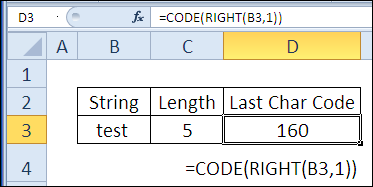
In cell D3, you can see that the last character of the string has the code 160, which corresponds to the non-breaking space that is used on websites.

Example 2: Finding the character code

To insert special characters in an Excel spreadsheet, you can use the command סימבאָל (Symbols) tab ינסערשאַן (Insert). For example, you can insert a degree symbol ° or copyright symbol ©.

Once a symbol has been inserted, its code can be determined using the function קאָד (KODSIMV):

=IF(C3="","",CODE(RIGHT(C3,1)))

=ЕСЛИ(C3="";"";КОДСИМВ(ПРАВСИМВ(C3;1)))

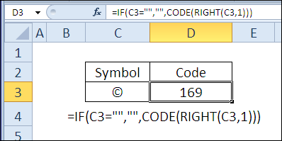
Now that you know the code, you can insert a character using the numeric keypad (not the numbers above the alphabetic keypad). Copyright symbol code − 169. Follow the steps below to enter this character into a cell.

Entering on the numeric keypad

1. דרוק דעם שליסל אַלט.
2. On the numeric keypad, enter the 4-digit code (if necessary, add the missing zeros): 0169.
3. לאָזן די שליסל אַלטto make the character appear in the cell. If necessary, press אַרייַן.

Keyboard input without number pad

In laptops, it happens that in order to use the functionality of the numeric keypad, you need to additionally press special keys. I recommend checking this with the user manual for your laptop. Here’s how it works on my Dell laptop:

1. דרוק אַ שליסל Fn און די F4, to turn on נומלאָקק.
2. Find the number pad located on the keys of the alphabetic keyboard. On my keyboard: די = 1, ק = 2 און אַזוי אויף.
3. גיט Alt+Fn and, using the numeric keypad, enter the 4-digit character code (adding zeros if necessary): 0169.
4. לאז גיין Alt+Fnto make the copyright symbol appear in the cell. If necessary, press אַרייַן.
5. When done, click again Fn+F4צו דיסייבאַל נומלאָקק.